All-Word-Embeddings-from-One-Embedding
All Word Embeddings from One Embedding
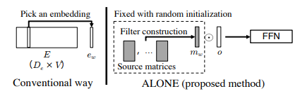
Embeddings are super important for neural networks as they do not understand categorial variables but only continuous ones. The way embedding matrices are constructed, in the traditional fashion, they scale somewhat linearly with the size of the input space which can get very memory heavy. Giving the size of the input space, $V$, and the embedding dimension, $D_e$, the conventional way does the one hot encoding as shown in the left figure below. The right figure represents the method ALONE (all word embeddings from one) that will be introduced in this blog.
However linear growth is also not always enough as the bigger input space might result in needing a bigger embedding dimension to contain all the information. In the English vocabulary there are around 200.000 words according to Wikipedia, where Korean has around 1.100.000 words. This means that the traditional embedding matrix for the English vocabulary would be $200.000\times D_e$ and $1.100.000\times D_e$ for Korean to set things in perspective. According to a Google developer blog from 2017 a general rule of thumb to find a fitting embedding dimension is: \(D_e = input\_space^{0.25}\) I.e. the fourth root of the input space. This would result in an embedding matrix with $200.000\times 21 = 4.200.000$ variables if training on the English vocabulary.
This paper by Takase and Kobayashi introduces a method to reduce the memory needed when having large input spaces. In order to reduce the memory they introduce the method ALONE which creates a shared embedding together with a small FFN and a non-trainable filter vector that is input specific.
Why could this be useful?
This is especially useful for me since my goal is to train a “next location” algorithm on big datasets for full countries/capitals which will need millions+ embeddings of specific locations that will generate big embedding matrices.
Do note that this is a simplification method, so having comparable results to state of the art is the goal and not necessary surpassing.
Method
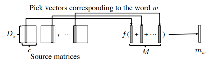
Instead of having an embedding matrix in the traditional size $(V\times D_0)$ Takase and Kobayashi introduce a shared trainable embedding vector $o\in \mathbb{R}^{1\times D_0}$. Takase and Kobayashi use this vector in combination with a word specific vector that they gather from a combination of M source matrices that are randomly initialized. Each word then uniformaly draws a random column from each source matrix and computes the sum of all the randomly drawn columns. Two filters are prposed which can then be used on this summation which gives the output $m_w$ as seen in the figure below. The element-wise product is then computed between $m_w$ and $o$, and then put through a small FFN to increase expressiveness of the output. In total the equation is: \(e_w=FFN(m_w \odot o)\) Where \(FFN(x)=W_2 (max(0,W_1 x)) \quad \text{and} \quad m_w=f\left(\sum_i^M m_w^i\right)\) With some filter function $f(x)$ that will be introduced in a bit. In the figure below the method for generating $m_w$ is illustrated visually.
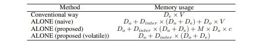
This method is only useful as long as $D_0,D_{inter},M\times c≪V$ such that memory is save. Since the Source matrices are randomly initialized and not trained they do not need to be saved as long as the random seed for generating them are saved. So if memory is very sparse the source matrices can be generated on the go. This might be computationally heavy but not saving them for production and only generating them on the go is a great benefit.
The table below shows the memory change where ALONE (proposed) is the method saving everything, and ALONE (proposed (volatile)) is the version that utilizes the fact that not all matrices have to be saved.
Takase and Kobayashi introduce two different filter functions, a binary mask filter and a real number vector filter.
Binary mask: A binary mask whose elements are 0 or 1 such that it ignore some of the elements in $o$. To achieve this Takase and Kobayashi suggests constructing the source matrices by sampling from the $Bernoulli(1−p_0^{1/M})$, and let the filter function $f$ be : \(Clip(a) = \begin{cases}1 & 1 \leq a \\ 0 & otherwise \end{cases}\) This will mask each value in $o$ with probability $p_0$.
Real number vector: A real number filter which is just the identity function, $f(x)=x$. Using this filter Takase and Kobayashi suggests using the Gaussian distribution to construct the source matrices.
Experiments:
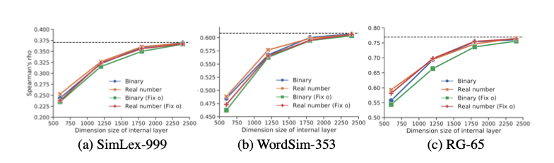
To test the flexibility of the method Takase and Kobayashi tried to mimic the GloVe embeddings with the ALONE method by trying to minimize the object function $\frac{1}{V}\sum_{w=1}^V|e_w−FFN(m_w\odot o)|^2$ where $e_w$ corresponds to the GloVe embedding of word $w$. Using the Spearman’s rank correlation to check on different datasets with GloVe they achieved the following convergence, which shows it succesfully mimics the GloVe embedding with less memory. Note this only shows that the method is complex enough to mimic already trained embeddings.
Results
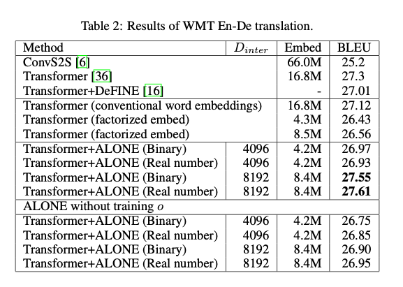
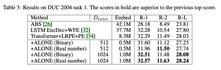
Testing ALONE together with known networks Takase and Kobayashi got the following results on translation from English to German. Included is the embedding sizes. Takase and Kobayashi show that using ALONE to train the embeddings they obtain similar scores to traditional methods while reducing the memory required. Other embeddings reduction methods are also included to give an idea of similarity. These methods are found to be a bit worse, but one should also keep in mind that they require extra training compared to ALONE.
What am I missing from the paper?
A great feature of training embeddings in the traditional way is how the embedding space can be trained to find underlying structures in the input space. I do not see them discovering if this method still retains this functionality in the same way.